Diffusion Models Beyond Images: Audio, Video, and 3D in 2026

If you only know diffusion models from image generators, you have seen the smallest version of what the technique now does. Diffusion models beyond images are the default architecture for almost every continuous-signal generation task in 2026: video, audio, music, speech, 3D shapes, and molecular structures all run on the same denoising idea that started with pictures. The pattern is consistent enough to be a rule of thumb. Where the data is continuous and high-dimensional, diffusion (paired with a transformer backbone) is the thing to beat. Where it is discrete and sequential, like text, autoregression still holds. Understanding why that line falls where it does, and what it costs to be on the diffusion side of it, is the practical core of this topic.

This is a builder's view, not a survey. The mechanics are shared across modalities, the engineering tradeoffs (especially latency) are where projects succeed or fail, and the model landscape moves fast enough that the durable knowledge is the shape of the technique, not this month's leaderboard.

One recipe, many modalities

The one idea, ported across modalities

A diffusion model learns to reverse a gradual corruption process. During training you take real data, add noise in many small steps until it is pure noise, and train a network to predict and remove that noise one step at a time. At generation, you start from random noise and run the learned denoiser repeatedly, each pass nudging the sample toward something that looks like real data. The reason this generalizes so well is that "add Gaussian noise, learn to remove it" makes no assumption about whether the data is pixels, audio samples, video frames, or point clouds. Swap the data and the backbone, keep the recipe.

Two refinements define the current generation. The backbone shifted from convolutional U-Nets to the diffusion transformer (DiT), which applies the transformer architecture to denoising and scales with data and compute the way transformers do everywhere else. And most production systems work in a compressed latent space rather than raw signal: an autoencoder maps the data down to a smaller latent, diffusion runs there, and a decoder maps back. Latent diffusion is what makes high-resolution video and long audio tractable, because the denoiser operates on a fraction of the dimensions.

The training objective also matured. The original formulation learned to predict the noise at each of many discrete timesteps, a noisy target that needed a lot of steps to integrate cleanly at generation. Flow matching reframes the problem as learning a direct velocity field from noise to data, a straighter path that trains more stably and, importantly for what comes later, needs fewer steps to traverse at inference. Flow matching is now the default objective for new large systems, and the reason is not aesthetic. A straighter path from noise to data is the same thing as a cheaper generation, which is the axis this entire field lives on.

Modality by modality

Video is where the technique is most visibly contested. The strong systems of 2026 (Google's Veo, Kuaishou's Kling, ByteDance's Seedance, and their peers) are all diffusion transformers operating in latent space, and the frontier moved from short, flickery clips to multi-second, temporally coherent, high-resolution shots. OpenAI's Sora was the early showcase that put the category on the map; by 2026 the active frontier is the Veo, Kling, and Seedance line, with Kling reaching native 4K at high frame rates and Seedance leaning into fine-grained, multi-input creative control. The defining recent shift is native audio-visual co-generation: rather than generating silent video and dubbing it, the model produces video and synchronized audio (dialogue, effects, ambient sound) jointly in a single pass. Veo introduced native audio in 2025, and by 2026 native audio went from a differentiator to a baseline expectation across the leaders, with competition moving to audio quality and lip-sync precision. This is the same territory the generative-simulator branch of world models is pushing into from the other side, and video is also where the cost is brutal, which the next section is about.

Audio, speech, and music run the same playbook on a one-dimensional signal (or a spectrogram). Diffusion produces high-fidelity text-to-speech and text-to-music, and the latent-diffusion trick applies directly: compress to a latent audio representation, denoise there, decode back to waveform. The quality ceiling for naturalness and timbre is high, and the same latency considerations apply, softened by the fact that audio latents are far smaller than video. That size difference is why real-time and near-real-time speech synthesis is a solved-enough problem in 2026 while real-time video is not: an audio latent for a few seconds of speech is a small tensor, so even a many-step sampler finishes fast, and a distilled few-step voice model runs comfortably inside an interactive loop. Music generation sits in between, because musical coherence over a full track demands a longer latent and more global structure than a single utterance.

3D and science are the frontier where diffusion does something autoregression has no natural way to do. Generating a 3D shape, a protein structure, or a small molecule means producing an object with no canonical ordering of its parts, and diffusion's "refine the whole object at once" process fits that better than "predict the next element in a sequence," which has to invent an order that does not exist. This is not a niche curiosity. Protein backbone design by diffusion (the RFdiffusion line of work) and the diffusion-based structure module inside AlphaFold3 are the reason structure generation moved from a research aspiration to a working tool, and molecular and materials generation follow the same pattern: define the object as a set of coordinates and types, corrupt it with noise, and learn to denoise back to a physically plausible configuration. For unordered, continuous, structured objects, the denoising formulation is a better match to the data than sequence prediction, and that is the deepest reason diffusion is not just an image trick.

The engineering problem: control and cost

Steering the denoiser: conditioning and guidance

None of this is useful if you cannot control what comes out, and control in diffusion works differently from a prompt to an autoregressive model. The condition (a text prompt, a reference image, an audio track, a pose skeleton) is fed into the denoiser, usually through cross-attention, so every denoising step is nudged toward outputs consistent with it. But conditioning alone is often too weak, and the lever that actually makes prompt adherence strong is classifier-free guidance. You train the model both with the condition and, some fraction of the time, without it, so it learns an unconditional and a conditional prediction. At generation you run both and push the sample away from the unconditional and toward the conditional by a guidance scale.

That scale is one of the most important knobs a builder touches, and it is a pure tradeoff. Turn it up and the output follows the prompt more tightly but loses diversity and starts to show artifacts (oversaturated images, over-smoothed audio, motion that snaps to the prompt at the cost of realism). Turn it down and the output is more varied and natural but drifts from what was asked. There is no universal right value; it is a per-model, per-task setting you tune on your own inputs. For spatial modalities, structural conditioning (the ControlNet family for images and video, driving generation from depth, edges, or pose) adds a second, geometric control channel on top of the text prompt.

The connection to the rest of this article is direct: classifier-free guidance means two forward passes per denoising step instead of one, so it doubles the cost of the exact loop that already dominates latency. That is why guidance distillation (baking the guidance behavior into a single network so you get the adherence without the second pass) is a standard part of the same few-step optimization the next section is about. Control and cost are not separate problems here; the knob that makes the output obey the prompt is also the knob that doubles the bill.

The latency tax is the whole engineering problem

The catch in every one of these modalities is the same, and it is the thing demos hide: diffusion generates by running the denoiser many times. A naive sampler needs tens to hundreds of forward passes through a large network to produce one output. For a single image that is seconds. For video, where each of those passes processes a stack of frames, it is the dominant cost and the reason video generation is slow and expensive, the same inference economics that govern LLM serving, amplified by the multi-step loop on top of an already-large model. An LLM pays for one forward pass per token; a diffusion model pays for tens of forward passes per output, and each pass is over the whole signal at once.

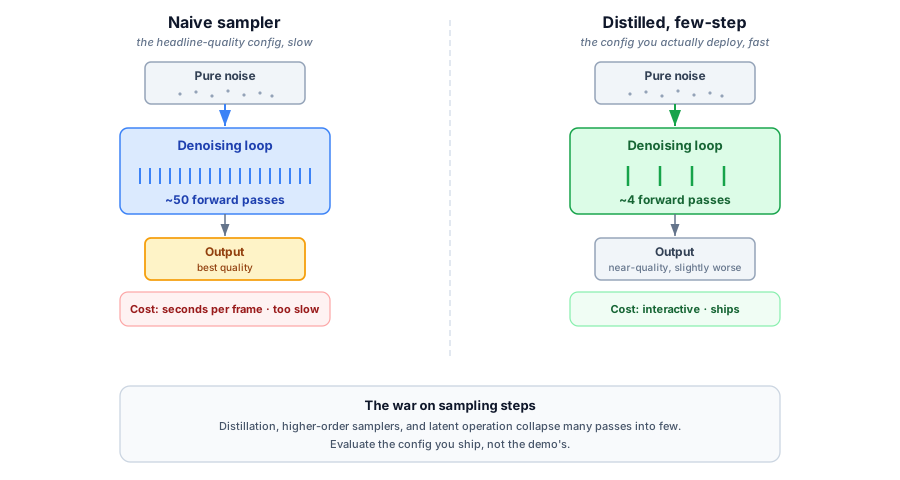
This is why the entire applied-diffusion field is, in practice, a war on sampling steps. The techniques that matter in production are the ones that cut the step count:

• Distillation trains a fast student to reproduce in a few steps what the teacher does in many. Consistency models and their latent successors learn to jump most of the way to the answer in one shot, pushing toward single or few-step generation and trading some quality for an order-of-magnitude latency cut. This is the single highest-leverage move in the field, because it attacks the multiplier directly.
• Better samplers (higher-order solvers for the underlying differential equation, the DPM-Solver family and its descendants) reach acceptable quality in fewer steps than the naive sampler, for free, with no retraining. A model that needed 50 steps with a first-order sampler often looks the same at 15 to 20 with a higher-order one.
• Latent-space operation (above) reduces the cost of each step rather than the number of steps, and composes with both of the above. A distilled model, on a good sampler, in a compressed latent, stacks all three savings.

The honest framing for a builder: the headline quality number comes from a slow, many-step configuration, and the deployable system runs a distilled or few-step version that is faster and slightly worse. Evaluate the configuration you will actually ship, not the one in the announcement, because the gap between "best quality" and "real-time" is exactly the step-count axis and it is where your cost and your user experience live. A useful discipline is to treat step count as a first-class deployment parameter and sweep it: measure quality at 50, 20, 8, and 4 steps on your own inputs, find the knee of the curve, and ship the point past which more steps buy nothing a user would notice.

Measuring generation honestly

Because the deployed system is not the demo system, evaluation is where most of the real disagreement lives, and it is easy to do badly. The automated metrics for generative media (FID for image distributions, FVD for video, and their relatives) compare the statistics of generated samples against a reference set, and they are useful for tracking a model against itself across training. They are far weaker as cross-model verdicts: they are sensitive to sample count, preprocessing, and the reference distribution, and a lower score is not a promise that humans prefer the output. Two models within a point or two on FVD can be clearly separable to a viewer, and clearly separable models can land close on the metric.

The reality-gap read is to treat a single headline metric on a slow config the way you would treat any leaderboard number: as a hypothesis, not a result. The number you should care about is a paired comparison at your deployed step count, on your input distribution, with human judgment on the axis your product actually sells (temporal coherence, lip-sync, prompt adherence, artifact rate), reported with enough samples to have an error bar. If a system's quality claim evaporates when you drop from the announcement's step count to the one you can afford, that is not a detail, that is the finding.

Where the line falls

Where autoregression still wins, and the diffusion-LM counterattack

The reality-gap discipline says name the boundary, so here it is. Text generation stays autoregressive (the reasoning-model line and essentially all production LLMs predict the next token) because language is discrete and sequential, and next-token prediction is both a natural fit and the substrate for the reasoning behaviors that emerged from scaling it.

The interesting part is that diffusion is genuinely attacking this turf, and the attack is real enough to take seriously. Diffusion language models generate a whole block of tokens in parallel and denoise it over a handful of passes instead of emitting one token at a time, and the payoff is throughput. Inception Labs' Mercury was the first commercially available diffusion LLM, and its 2026 successor reports on the order of a thousand tokens per second on a single current-generation GPU, several times faster than similarly-sized autoregressive models on the same hardware. Open research models like the LLaDA line showed the approach trains at 8B scale and, in later versions, is being pushed toward 100B-scale feasibility, and Google's Gemini Diffusion demonstrated the same parallel-generation speed advantage inside a frontier lab. On code and structured output, where the target has strong local structure and a fixed shape, these speeds are not a trick, they are a real latency win.

But look at how the production-grade versions actually work, because it is the most honest thing in this whole area. The design that made diffusion LMs deployable is block diffusion: instead of denoising an entire response in parallel, the model generates in blocks (a small window of tokens at a time), applies diffusion within each block, and moves left to right across blocks. That last clause is the tell. Block diffusion re-imports autoregressive structure, generating blocks in sequence, precisely because pure parallel generation gave up the two things autoregression gets for free: a KV cache to reuse across the sequence, and flexible output length. The winning diffusion-LM design is the one that looks most like autoregression, and the dominant training recipe underlines the point, since the compute-efficient way to build one in 2026 is to initialize from a pretrained autoregressive model and continue training it with the diffusion objective rather than train from scratch. The counterattack is real, and its most successful form is a hybrid that concedes the sequential structure it set out to replace.

So the honest boundary is not "text is forever autoregressive." It is narrower and more useful: for latency-bound generation of structured, bounded-length text like code, a block-diffusion model is a legitimate and sometimes winning choice, and worth evaluating against an autoregressive baseline on your own task with a real acceptance-quality comparison, not a tokens-per-second headline. For open-ended reasoning, long-form generation, and anything where the length is not known in advance and the value is in a chain of dependent steps, autoregression still holds, because next-token prediction carries the reasoning machinery and does not have to guess how long the answer will be. Treating "diffusion is winning everywhere" as settled is exactly the overclaim to avoid.

The clean way to hold all of it: diffusion dominates continuous, high-dimensional, order-free generation (images, audio, video, 3D, molecules) because parallel whole-object refinement matches that data. Autoregression dominates discrete, sequential, open-ended generation (general text, reasoning) because next-element prediction matches that data and carries the reasoning behaviors. The contested middle (diffusion for text, autoregression for images) is where each is trying to take the other's home turf, and where you should read claims skeptically and ask what was measured against the incumbent on its own ground, at a deployable config. For the non-text modalities this article covers, the verdict is not contested: in 2026, diffusion is the default, and the engineering question is not whether to use it but how few steps you can get away with.

Key Takeaways

1. Diffusion is the default for continuous signals. Audio, video, music, speech, 3D, and molecules all run on the same denoising recipe that started with images, because "add noise, learn to remove it" makes no assumption about the data type.
2. The backbone is now the transformer, trained by flow matching. Diffusion transformers (DiT) replaced U-Nets and scale with data and compute the way transformers do elsewhere; most systems denoise in a compressed latent space, and flow matching is now the default objective because a straighter noise-to-data path is a cheaper generation.
3. Video is the contested showcase. Veo, Kling, Seedance, and their peers are all latent diffusion transformers, and native audio-visual co-generation (joint video plus synchronized audio in one pass) went from differentiator to baseline by 2026.
4. 3D and science are the deepest fit. For objects with no natural ordering (shapes, proteins, molecules), whole-object refinement beats next-element prediction, which would have to invent an order that does not exist. Protein design (RFdiffusion) and AlphaFold3's structure module are the working proof.
5. The latency tax is the core engineering problem. Diffusion runs the denoiser many times per output, which dominates cost for video. The applied field is largely a war on sampling steps.
6. Step reduction is how it ships. Distillation and consistency models cut steps toward single-digit counts; higher-order samplers cut steps for free; latent operation cuts per-step cost. Production runs a faster, slightly-worse configuration than the headline.
7. Evaluate the config you will deploy, honestly. The quality number comes from a slow many-step setup on a metric like FVD that is weak as a cross-model verdict; the real system is the distilled few-step one. Sweep step count on your own inputs and judge with human comparison at the config you can afford.
8. Autoregression still owns open-ended text, and diffusion's best counterattack proves it. Diffusion LMs (Mercury, LLaDA, Gemini Diffusion) are real and fast on structured output, but the deployable design (block diffusion) works by re-importing autoregressive structure. The verdict is modality-specific, not universal.

The Acing AI newsletter covers generative models for the part that decides deployment: the latency, the step count, and the configuration you actually ship. Subscribe for the grounded version.